Bunching of Numbers in a Non-Ideal Roulette: The Key to Winning Strategies
Chances of a gambler are always lower than chances of a casino in the case of an ideal, mathematically perfect roulette, if the capital of the gambler is limited and the minimum and maximum allowed bets are limited by the casino. However, a realistic roulette is not ideal: the probabilities of realisation of different numbers slightly deviate. Describing this deviation by a statistical distribution with a width δ we find a critical δ that equalizes chances of gambler and casino in the case of a simple strategy of the game: the gambler always puts equal bets to the last N numbers. For up-critical δ the expected return of the roulette becomes positive. We show that the dramatic increase of gambler’s chances is a manifestation of bunching of numbers in a non-ideal roulette. We also estimate the critical starting capital needed to ensure the low risk game for an indefinite time.
Roulette is one the most famous games of hasard. It is equally famous as a mathematical toy model. In a European roulette, which we mostly discuss in this Letter, a croupier spins a wheel in one direction, then spins a ball in the opposite direction around a tilted circular track running around the circumference of the wheel. The ball eventually loses momentum and falls onto the wheel and into one of 37 colored and numbered pockets on the wheel [1]. It has been shown a long time ago that a casino has always better chances than a gambler for the simple reason that the probability of realisation of any number is 1/37, while in the case of win the gambler collects his/her bet times 36 (for a recent review see [2]). In the American roulette, the chances of a gambler are even lower as the wheel has 38 sectors (numbers from 0 to 36 and the double zero sector), while betting on a number a player only collects 36 times the bet in the case of win. Multiple strategies have been invented over centuries to circumvent this simple mathematics that necessarily gives better chances to a casino than to a gambler [3]. As an example, the popular martingale strategy relies on the game of chances (e.g. red and black), where the bet is doubled in case of loss. The probability to win is 18/37 < 1/2 each time, while gamblers try to increase their chances by doubling their bets after each loss and coming back to the initial bet after each win. Clearly, on a long time scale this strategy may only work if the capital of the gambler is unlimited and the casino imposes no limits to the bets, that is never the case. Other strategies are based on an intuitive feeling of gamblers that a roulette might have memory. Assuming this, they believe that if e.g. “red” came 10 times in row; there is a higher probability for “black” to come on the 11th spin, as the system must tend to equalize the number of black and red outcomes. As there is no any rational reason for roulette to have memory, this strategy is doomed to fail on a long time-scale. In a similar way, none of “winning strategies” may provide better chances to a gambler than to a casino on a long time-scale (number of spins tending to infinity). If a gambler has an initial capital C his/her chances to double this capital are lower than the chances to lose it by at least 1/37 independently of the adapted strategy.
Still, there are professional roulette players who manage to collect steady profits from their matter. They exploit deviations of all realistic mechanical roulettes from the ideal. These deviations may be caused by the geometry of the roulette, correlation between the speed of spinning and the initial velocity of the ball, as well as by human factors: a croupier is not a random number generator, after all. Some well-trained croupiers may want sending balls to preselected sectors of the wheel on purpose of overplaing gamblers who place their bets in opposite sectors. All these factors result in a non-uniform distribution of probabilities for realisation of different numbers.
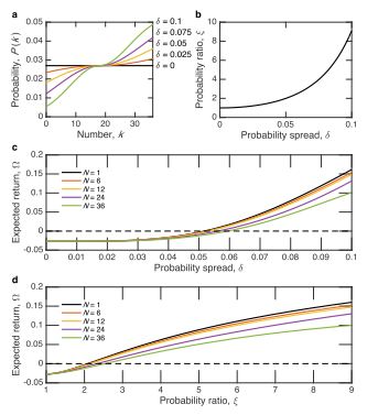
Let us assume that the distribution of probabilities is a smooth function with the maximum at 1/37 and Gaussian tails. Later we shall also consider a linear distribution function for the sake of comparison (Figure 1). Renumbering all numbers of the roulette in the order of increasing probability of realisation, k = 0, 1, . . . , 36 we set the probability for the
number k to be realised as
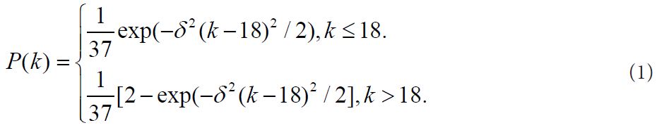
k = 0 has the lowest probability with P(0) = (1/37) exp(−162δ2), k = 36 has the highest probability with P(36) = 2/37 − P(0) and P(18) = 1/37 for any δ. In Figure 1(a), we show the probability distribution P(k) for different values of δ. It is instructive to consider also the ratio between the highest and the lowest probability:
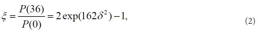
which is shown in Figure 1(b). The following formalism is independent of the specific shape of P(k), while, of course, the numerical results may be affected by the choice of P(k), as discussed below.
We underline that the correspondence between the numbers k and the real numbers on the roulette wheel is unknown to us, and we do not intend to know it. Frequently, experienced gamblers try to collect statistics of realisation of different numbers over several hundred spins, select “happy” numbers and then keep steadily playing on these numbers. This is a time consuming method that sometimes meets disapproval by casino administrations. Moreover, test measurements for “happy numbers” need to be re-done frequently, as e.g. croupier gets replaced, speed of spinning may be reset etc. A much simpler method suitable for an amateur consists in betting on the last sequence of numbers realized. Many casinos display the last numbers for the convenience of gamblers. We shall consider the case of a gambler with a sufficient starting capital always playing the last N numbers placing equal bets on each Number. The advantage of this method is that it does not rely on any statistics collected previously and easily adapts to the changes imposed by the casino.
Here we prove that the method may be also considered as a convenient tool for the measurement of the parameters δ and ξ characterising the distribution of probabilities. In particular, we shall be looking for the critical value of δ or ξ that provides a sufficient bunching of numbers which equalizes the chances of gambler and casino. Let us assume that the latest N numbers chosen by a roulette are k1, k2, ..., kN . We will call this sequence nth realisation. We note that some of these numbers may coincide. The probability of nth realisation is given by  . We shall assume that there are jn different numbers among the last N numbers. jn varies from 1 to N. The probability to have on the (N + 1)st position one of the numbers ki (i = 1, 2, ..., N) is given by
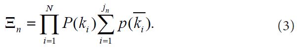
  Here, ki denote those jn numbers that are different among N last numbers. Hence, the probability to have first the sequence k1, k2, ..., kN and then one of the numbers ki , (i = 1, 2, ..., N) is given by
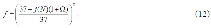
Now, in order to find the probability of this event, we need to sum Ξn over all possible sequences. This yields:
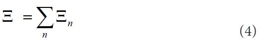
This sum has 37N elements. One can easily find the expected return of the roulette, Ω, as
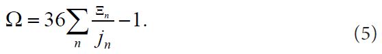
In order to analyze the chances of a gambler to have an advantage over casino, let us start from the critical spread of the probability distribution δ which equalises the chances of casino and gambler. It is given by a condition:

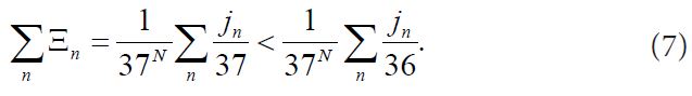
An important particular case is the limit of an ideal roulette. In this case δ = 0, P(k) = 1/37 for all k,  . Clearly, in this case the casino has an advantage over the gambler as
In this limit, the expected return of the roulette Ω0 is well known:

Another limit is of δ = ∞ that corresponds to a zero probability of realisation of all numbers with k < 18, P(18) = 1/37 and P(k > 18) = 2/37. In this case the gambler always wins with the adapted method. In Figure 1(c,d), we show the results of Monte-Carlo simulations of the expected return of the roulette Ω(δ) and Ω(ξ), respectively, calculated for different values of N [4]. We have used a standard generator of a sequence of uniformly distributed random numbers, and run 106 realisations for each point [5]. One can see that starting from δ ≈ 0.05 a gambler has an advantage over the casino for a wide range of N. This critical value of δ corresponds to the ratio of probabilities of the realisation of the highest probable and the lowest probable numbers of ξc ≈ 2.012.
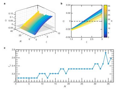
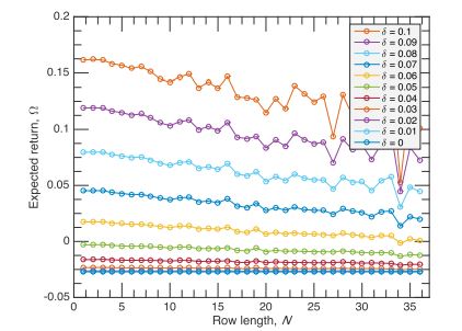
Figure 2(a) is a 3D plot showing Ω(N, ξ). From the 2D plot of the same function shown in Figure 2(b) one can see that, in general, Ω slightly decreases with the increase of N, and a gambler can have an advantage over the casino for a wide range of N if δ > 0.05 (ξ > 2). Figure 2(c) shows ξc that provides the expected return Ω = 0 as a function of N. The dependence of Ω on N is important and needs further analysis. In Figure 3, we show the results of Monte-Carlo simulations of the expected return Ω as a function of N for different values of the probability spread δ. One can see that for small δ the expected return does not show any appreciable dependence on N, while for larger δ the expected return slightly decreases with the increase of N. It looks like the choice of a relatively small N is the best. However, as we will below, small N strategies are more risky in terms of a probability of critical fluctuations that would consume the entire capital of the gambler.
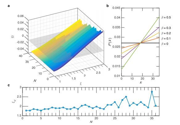
In order to check the robustness of our method, we have also run the simulations for the expected return using a simplest linear probability distribution function:
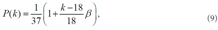
where β is a parameter describing the spread of the probability. In this case,
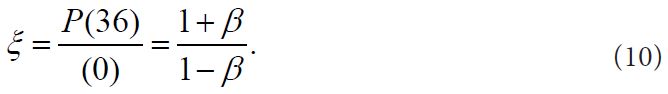
Figure 4(a) shows the 3D plot Ω(N, ξ) calculated using the probability function (9). Qualitatively, the results of the modeling are similar to those obtained with the Gaussian distribution. Indeed, the spread of probabilities results in bunching of numbers, so that a gambler playing on the last N numbers may have an advantage over casino. The critical value of ξ that corresponds to Ω = 0 is close to 2 similarly to the results obtained with the distribution function (1). The dependence of Ω on N is very weak, within the statistical noise produced by our Monte-Carlo simulator.
Finally, note that our analysis can be easily generalised for the case of an American roulette by replacing 37 by 38 in the above formalism. Obviously, the critical value of δ would be higher for the American roulette as compared to the European roulette.
For the practical implementation of the strategy described here, it is important to know the value of an initial capital that assures successful gambling. We recall that in the case of an ideal roulette that is characterised by a negative Ω ≈ −0.027 for any finite starting capital the gambler loses after a sufficiently large number of bets. In our case, Ω > 0, and the capital of a gambler normally increases in the course of the game. However, the risk is also present: due to a negative fluctuation (sequence of lost spins) the gambler can lose his/her capital and be put out of a game. What should be the size of the initial capital that ensures the relatively safe game and reduces the risk of catastrophic negative fluctuations? While it is impossible to exclude a catastrophic fluctuation entirely, one can introduce such a characteristic (critical) value of the initial capital C. We define C. as a capital that allows a gambler to double it during the average number of spins M that elapses between two catastrophic fluctuations. A catastrophic fluctuation is defined as a loss of C. in a sequence of unsuccessful spins. We note at this point that for an ideal roulette Finally, note that our analysis can be easily generalised for the case of an American roulette by replacing 37 by 38 in the above formalism. Obviously, the critical value of δ would be higher for the American roulette as compared to the European roulette

where  is the average value of different numbers among the last N numbers. Now, the frequency of catastrophic fluctuations is given by
where S is the number of successive unsuccessful spins needed to lose the capital C. As each next unsuccessful spin increases our loss by , in average, we obtain:

Now, M is linked with the frequency of catastrophic events by

Expressing M and S in terms of C with use of Eqs. (11) and (13), we obtain the transcendental equation for the critical capital:
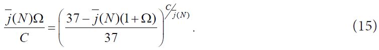
Here, C is expressed in units of bets. To be on a safe side, a gambler should possess a capital exceeding C.
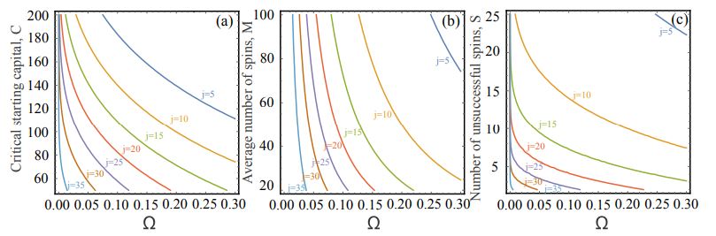
Figure 5 shows the dependences of C and corresponding values of M and S on Ω calculated for different values of the average number of bets per spin . One can see that C strongly decreases with the increase of both Ω and .
This is important for a gambler who aims at following the safetest strategy, while willing to achieve significant benefits nevertheless. One should keep in mind also that Ω slightly decreases as a function of N, while is a monotonically increasing function. Clearly, playing on a larger series of latest numbers N one can strongly reduce the risk of a catastrophic fluctuation. The price to pay is a simultaneous decrease of the expected return. The most convenient range of N is likely to be between 10 and 20 for a sufficiently high δ (δ is of the order of 0.1). Note also that the avarage number of spins separating two negative fluctuations which lead to the loss of the initial capital, M, as well as the number of successive unsucessful spins needed to exhaust this capital, S, linearly increase with the increase of C, as Figure 5(b,c)) shows. Both quantities decrease with the increase of the expected return Ω and with the increase of the average number of bets per spin .
The strategy described here has been tested on three European roulette tables in two different casinos of Southampton (UK) on several different days. We have played N = 12 in one casino and N = 17 in another one: in order to try the sufficiently different strategies and check the robustness of the developed method. In both cases the results were steadily positive with Ω ≈ 0.1 independently on croupier. The statistics has been taken over several hundred of spins. For evident reasons, we did not inform administration of the casinos of our experiments, which could have been run without any external bias. The tests have been realised with minimum allowed bets and all the money won in this way were donated to charity.
To conclude, our analysis shows that certain strategies may result in the positive expected return in the case of a non-ideal roulette. Our method of playing on the last N numbers does not require any preliminary knowledge on “hot” or “cold” numbers, speed of the ball, speed of the wheel etc. The outcome of a long game is only dependent on the value of the probability spread parameters δ or ξ and on the chosen value of N. We show also that while the expected return of a non-ideal roulette shows only a weak dependence on N (it slightly decreases with the increase of N), a gambler may significantly reduce the risk of a catastrophic loss if playing on a longer sequence of numbers. In practical terms, we would recommend a gambler to play the strategy described here with any unknown roulette by initially placing only minimum bets for the first 100 or 200 spins (the higher N is chosen the lower number of spins is needed). If the outcome turns out to be steadily positive, it means that, most likely, δ is above critical. Once all doubts are left behind, the gambler may start placing maximum bets that would bring him a significant benefit. If, when placing minimum bets for 100 or 200 spins the gambler does not see any sign of a steadily positive tendency, the chosen roulette is probably close to ideal, and there is no reason to continue playing on this roulette. We also warn that the positive expected return does not guarantee a gambler against the loss due to a negative fluctuation and advice against irresposible gambling.
AK acknowledges support from the EPSRC Established Career fellowship. MP acknowledge financial support from Saint-Petersburg State University (Research Grant No. 11.34.2.2012). ASS acknowledges ITMO Fellowship and Visiting Professorship. The work was carried out with financial support from the Ministry of Education and Science of the Russian Federation in the framework of increase Competitiveness Program of NUST MISIS, implemented by a governmental decree dated 16th of March 2013, No 211.