Conditioning Gaussian Measure on Hilbert Space

---

For a Gaussian measure on a separable Hilbert space with covariance operator C, we show that the family of conditional measures associated with conditioning on a closed subspace S⊥ are Gaussian with covariance operator the short S(C) of the operator C to S. Although the shorted operator is a well-known generalization of the Schur complement, this fundamental generalization to infinite dimensions of the well-known relationship between the Schur complement and the covariance operator of the conditioned Gaussian measure is new. Moreover, the conditioning of infinite dimensional Gaussian measures appears in many fields so that this simply expressed result appears to unify and simplify these efforts.

We provide two proofs. The first uses the theory of Gaussian Hilbert spaces and a characterization of the shorted operator by Andersen and Trapp. The second uses recent developments by Corach, Maestripieri and Stojanoff on the relationship between the shorted operator and C-symmetric projections onto S⊥. To obtain the assertion when such projections do not exist, we develop an approximation result for the shorted operator by showing, for any positive operator A, how to construct a sequence of approximating operators An which possess An-symmetric oblique projections onto S⊥ such that the sequence of shorted operators S(Aⁿ) converges to S(A) in the weak operator topology. This result combined with the martingale convergence of random variables associated with the corresponding approximations Cn establishes the main assertion in general. Moreover, it in turn strengthens the approximation theorem for shorted operator when the operator is trace class; then the sequence of shorted operators S(Aⁿ) converges to S(A) in trace norm.

Keywords:Conditioning; Gaussian Measure; Hilbert Space; Shorted Operator; Schur; Oblique Projection; Infinite Dimensions

AMS subject classifications:60B05, 65D15

For a Gaussian measure μ with injective covariance operator C on a direct sum of finite dimensional Hilbert spaces , the conditional measure associated with conditioning on the value of H₂ can be computed in terms of the Schur complement corresponding to the partitioning of the covariance matrix C. Evidently, the natural extension to infinite dimensions of the Schur complement is the shorted operator, first discovered by Krein and developed in Anderson and Trapp [1,2]. However, the connection between the shorted operator and the covariance operator of the conditional Gaussian measure on an infinite dimensional Hilbert space appears yet to be established. Indeed, Lemma 4.3 of Hairer, Stuart, Voss, and Wiber, see also Stuart, characterizes the conditional measure through a measurable extension result of Dalecky and Fomin of an operator defined on the CameronMartin reproducing kernel Hilbert space [3-5]. For other representations, see Mandelbaum, and Tarieladze and Vakhania’s extension of the optimal linear approximation results of Lee and Wasilkowski from finite to infinite rank, extending results in the Information-Based Complexity of Traub, Wasilkowski and Wozniakowski [6-10].

The primary purpose of this paper is to demonstrate that, for a Gaussian measure with covariance operator C, the covariance operator of the Gaussian measure obtained by conditioning on a subspace is the short of C to the orthogonal complement of that subspace. We provide two distinct proofs. The first uses the theory of Gaussian Hilbert spaces and a characterization of the shorted operator by Andersen and Trapp. The second proof, corresponding to the secondary purpose of this paper, uses recent developments by Corach, Maestripieri and Stojanoff on the relationship between the shorted operator and A-symmetric oblique projections. This latter approach has the advantage that it facilitates a general approximation technique that not only can be used to approximate the covariance operator but the conditional expectation operator. This is accomplished through the development of an approximation theory for the shorted operator in terms of oblique projections followed by an application of the martingale convergence theorem. Although the proofs are not fundamentally difficult, the result (which appears to have been missed in the literature) provides a simple characterization of the conditional measure, leading to significant approximation results. For instance, the attainment of the main result through the martingale approach feeds back a strengthening of the approximation theorem for the shorted operator that was developed for that purpose: when the operator is trace class the approximation improves from weak convergence to convergence in trace norm.

Conditioning Gaussian measures has applications in Information-Based Complexity and, beginning with Poincare, publications by e.g. Diaconis, Sul’din, Larkin, Sard, Kimeldorf and Wahba, Shaw, and Hagan they have been useful in the development of statistical approaches to numerical analysis [10-18]. Although they received little attention in the past, the possibilities offered by combining numerical uncertainties/errors with model uncertainties/errors are stimulating the reemergence of such methods and, as discussed in Briol et al. and Owhadi and Scovel, the process of conditioning on closed subspaces is of direct interest to the reemerging field of Probabilistic Numerics where solutions of PDEs and ODEs are randomized and numerical errors are interpreted in a Bayesian framework as posterior distributions [19-31] Furthermore, as shown in Gaussian measures are a class of optimal measures for minmax recovery problems emerging in Numerical Analysis (when quadratic norms are used to define relative errors) and conditioning such measures on finite-dimensional linear projections lead to the identification of scalable algorithms for a wide range of operators[20,32]. Representing the process of conditioning Gaussian measures on closed (possibility infinite dimensional) subspaces via converging sequences of shorted operators, could be used as a tool for reducing/compressing infinite-dimensional operators and identifying reduced models. In particular, it is shown in that the underlying connection with Schur complements can be exploited to invert and compress dense kernel matrices appearing in Machine Learning and Probabilistic Numerics in near linear complexity, thereby opening the complexity bottleneck of kernel methods [31].

Let us review the basic results on Gaussian measures on Hilbert space. A measure μ on a Hilbert space H is said to be Gaussian if, for each hH considered as a continuous linear function h: H →R by we have that the pushforward measure h*μ is Gaussian, where we say that a Dirac measure is Gaussian. For a Gaussian measure μ, its mean m is defined by

and its covariance operator C : H →H is defined by

A Gaussian measure has a well defined mean and a continuous covariance operator, see e.g. Da Prato and Zabczyk [33]. Mourier’s Theorem, see Vakhania, Tarieladze and Chobanyan, asserts, for any mH and any positive symmetric trace class operator C, that there exists a Gaussian measure with mean m and covariance operator C, and that all Gaussian measures have a well defined mean and positive trace class covariance operator. This characterization also follows from Sazonov’s Theorem [34].

Since separable Hilbert spaces are Polish, it follows from the product space version, see e.g. Dudley, of the theorem on the existence and uniqueness of regular conditional probabilities on Polish spaces, that any Gaussian measure μ on a direct sum of separable Hilbert spaces has a regular conditional probability, that is there is a family μt , tH₂ of conditional measures corresponding to conditioning on H₂. Moreover, Tarieladze and Vakhania demonstrate that the corresponding family of conditional measures are Gaussian[8,35]. Bogachev’s theorem of normal correlation of Hilbert space valued Gaussian random variables shows that if two Gaussian random vectors ξ and η on a separable Hilbert space H are jointly Gaussian in the product space, then E[ξ|η] is a Gaussian random vector and ξ =E[ξ|η]+ζ where ζ is Gaussian random vector which is independent of η. Consequently, for any two vectors h₁,h₂H we have

and so we conclude that, just as in the finite dimensional case, the conditional covariance operators are independent of the values of the conditioning variables [36].

Since both proof techniques will utilize the characterization of conditional expectation as orthogonal projection, we introduce these notions now. Consider the Lebesgue Bochner space L² (H,μ,(H)) space of (equivalence classes) of H-valued Borel measurable functions on H whose squared norm

is integrable. For a sub σ-algebra of the Borel σ-algebra, consider the corresponding Lebesgue-Bochner space L²(H,μ,Σ). As in the scalar case, one can show that are Hilbert spaces and that is a closed subspace. Then, if we note that contractive projections on Hilbert space are orthogonal, it follows from Diestel and Uhl that conditional expectation amounts to orthogonal projection [37].

A symmetric operator A: H →H is called positive if(Ax,x)≥0 for all x∈H. We denote by L₊(H) the set of positive operators and we denote such positivity by A≥0. Positivity induces the (Loewner) partial order ≥ on L₊(H). For a closed subspace S H and a positive operator A L₊(H) consider the set

Then Krein and later Anderson and Trapp showed that H(A,S) contains a maximal element, which we denote by S(A) and call the short of A to S. For another closed subspace TH, we denote the short of A to T by T (A). In the proof, Anderson and Trapp [1] demonstrate that when A is invertible, that in terms of its (S,S^⊥) partition representation [1,2].

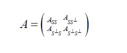
that is invertible and

It is easy to show that the assertion holds under the weaker assumption that be invertible. Moreover, Anderson and Trapp asserts for A,B L+(H), that

that is, S is monotone in the Loewner ordering, and for two closed subspaces S and T, we have

Finally, Theorem 6 of Anderson and Trapp asserts that if A: H →H is a positive operator and S⊂H is a closed linear subspace, then

In Section 4.1 we demonstrate how the characterization (2.1) of the shorted operator combined with the theory of Gaussian Hilbert spaces provides a natural proof of our main result, the following theorem. Here we consider direct sum split and let S = H₁ and S^⊥ = H₂, so that the short S(A) of an operator to the subspace S = H₁ will be written as H₁(A).

Theorem 2.1. Consider a Gaussian measure μ on an orthogonal direct sum of separable Hilbert spaces with mean m and covariance operator C. Then for all t H₂, the conditional measure μt is a Gaussian measure with covariance operator H₁(C).

In this section, we will prepare for an alternative proof of Theorem 2.1 using oblique projections along with the development of approximations of the covariance operator and the conditional expectation operator generated by natural sequences of oblique projections. To that end, let us introduce some notations. For a separable Hilbert space H, we denote the usual, or strong, convergence of sequences by h_n →h and the weak convergence byh_n^ω→Let L(H) denote the Banach algebra of bounded linear operators on H. For an operator A L(H), we let R(A) denote its range and ker(A) denote its nullspace. Recall the uniform operator topology on L(H) defined by the metric We say that a sequence of operators Aⁿ L(H) converges strongly to A L(H), that is

if Aⁿh→Ah for all h∈ H, and we say that Aⁿ →A weakly or

if for all hH. Recall that an operator AL(H) is called trace class if the trace norm

is finite for some orthonormal basis, where is the absolute value. When it is finite, then is well defined, and for all positive trace class operators A we have 1. The trace norm ||.||₁ makes the subspace of trace class operators into a Banach space. It is well known that the sequence of operator topologies

weak→strong→ uniform operator→trace norm

increases from left to right in strength.

For a positive operator A: H →H, let us define the set of (A-symmetric) oblique projections

onto S^⊥, where Q^* is the adjoint of Q with respect to the scalar product<·,·>on H. The pair (A, S^⊥) is said to be compatible, or S⊥ is said to be compatible with A, if P(A, S^⊥) is nonempty. For any oblique projection QP(A, S^⊥), Corach, Maestripieri and Stojanoff asserts that for E := 1−Q, we have

Moreover,when (A,S^⊥) is compatible, according to Corach, Maestripieri and Stojanoff,there is a special element defined in the following way: by their Proposition 3.3 and their factorization Theorem 2.2 there is a unique operator which satisfies such that ker needs overbar Defining

their Theorem 3.5 asserts that

When the pair (A,S^⊥) is not compatible, we seek an approximating sequence An to A which is compatible with S^⊥, such that the limit of S(An) is S(A). Although Anderson and Trapp show that if Aⁿ is a monotone decreasing sequence of positive operators which converge strongly to A, that the decreasing sequence of positive operators S(An) strongly converges to S(A), the approximation from above by Aⁿ:=A+1/nI determines operators which are not trace class, so is not useful for the approximation problem for the covariance operators for Gaussian measures. Since the trace class operators are well approximated from below by finite rank operators one might hope to approximate A by an increasing sequence of finite rank operators. However, it is easy to see that, in general, the same convergence result does not hold for increasing sequences. The following theorem demonstrates, for any positive operator A, how to produce a sequence of positive operators Aⁿ which are compatible with S^⊥ such that S(Aⁿ) weakly converges to S(A)[2,38].

Henceforth we consider a direct sum split , and let S = H₁ and S^⊥ = H₂, so that the short S(A) of an operator to the subspace S = H¹ will be written as H¹(A). Let us also denote by Pⁱ: H →H the orthogonal projections onto Hⁱ, for i= 1,2, and let Πⁱ : H →Hⁱ denote the corresponding projections and Π^*_i: H_i →H, the corresponding injections. For any operator A: H→H, consider the decomposition

where the components are defined by A_ij:=AΠ^*_i,i,j=1,2.

Theorem 3.1. Consider a positive operator A: H →H on a separable Hilbert space. Then for any orthogonal split and any ordered orthonormal basis of H₂ⁿ,we let denote the span of the first n basis elements and let p p p denote the orthogonal projection onto Then the sequence of positive operators

is compatible with H₂ and

Remark 3.2. For an increasing sequence An of positive operators converging strongly to A, the monotonicity of the shorting operation implies that the sequence H₁(Aⁿ) is increasing, and therefore Vigier’s Theorem implies that the sequence H₁(Aⁿ) converges strongly. Although the sequence Aⁿ:=PⁿAPⁿ defined in Theorem 3.1 is positive and converges strongly to A, in general, it is not increasing in the Loewner order, so that Vigier’s Theorem does not apply, possibly suggesting why we only obtain convergence in the weak operator topology. With stronger assumptions on the operator A and a well chosen selection of an ordered orthonormal basis of H₂, we conjecture that convergence in a stronger topology may be available. In particular, as a corollary to our main result, when A is trace class, we establish in Corollary 3.4 that

H₁(An)→H₁(A) in trace norm.

For any mH, we let m= (m₁,m₂) denote its decomposition in Moreover, for any projection Q: H →H with R(Q) = H₂ we let denote the unique operator such that

and denote by the adjoint of defined by the relation

The following theorem constitutes an expansion of our main result, Theorem 2.1, to include natural approximations for the conditional covariance operator and the conditional expectation operator.

Theorem 3.3. Consider a Gaussian measure μ on an orthogonal direct sum of separable Hilbert spaces with mean m and covariance operator C. Then for all tH₂,the conditional measure μ_t is a Gaussian measure with covariance operator H₁(C).

If the covariance operator C is compatible with H₂, then for any oblique projection Q in, the mean mt of the conditional measure μ_t is

In the general case, for any ordered orthonormal basis for H₂, let H₂ⁿ denote the span of the first n basis elements, let p p p denote the orthogonal projection onto and define the approximate Cⁿ:=PⁿCPⁿ. Then Cn is compatible with H₂ for all n, and for any sequence Q_n P(C_n,H₂) ≠ Ø of oblique projections, we have

for μ-almost every t. If the sequence Q_n eventually becomes the special element Q_n=Q_Cⁿ,H2 defined near (3.2), then we have

for μ-almost every t.

As a corollary to Theorem 3.3, we obtain a strengthening of the assertion of Theorem 3.1 when the operator A is trace class.

Corollary 3.4. Consider the situation of Theorem 3.1 with A trace class.Then

H₁(Aⁿ )→H₁(A) in trace norm

First proof of Theorem 2.1 Consider the Lebesgue-Bochner space space of (equivalence classes) of H-valued Borel measurable functions on whose squared norm

is integrable. For any square Bochner integrable function and any hH, we have that is square integrable, that is Moreover, it is easy to see that if f is Bochner integrable, then for all hH, we have is Bochner integrable and

Now consider the orthogonal decomposition and the Borel σ-algebra (H₂). Let us denote the shorthand notation

The definition of conditional expectation in Lebesgue-Bochner space, that is that is the unique μ-almost everywhere ₂-measurable function such that

combined with Hille’s theorem [13,Thm. II.6], that for each hH we have

and

implies that

thus implying the following commutative diagram for all h H:

When μ is a Gaussian measure, the theory of Gaussian Hilbert spaces, see e.g. Jansen, provides a stronger characterization of conditional expectation of the canonical random variable X(h):=h,hH when conditioning on a subspace and captures the full linear nature of Gaussian conditioning [39]. Let us assume henceforth that μ is a centered Gaussian measure. Then Fernique’s Theorem, see Theorem 2.6 in Da Prato, implies that the random variable X is square Bochner integrable [33]. For any element hH, let us denote the corresponding function ξ_h : H →R defined by Then the the discussion above shows that for any hH, that the real-valued random variable ξ_h is square integrable, that is ξ_hL² (R,μ,), for all hH. Let

denote the resulting linear mapping defined by

It is straightforward to show that ξ is injective if and only if the covariance operator C of the Gaussian measure μ is injective. By the definition of a centered Gaussian vector X, it follows that the law (ξ_h)_*μ in R is a univariate centered Gaussian measure, that is ξ_h is a centered Gaussian real-valued random variable. Consequently, let us consider the closed linear subspace

generated by the elements By Theorem I.1.3 of Jansen, this closure also consists of centered Gaussian random variables, and since it is a closed subspace of a Hilbert space, it is a Hilbert space and therefore a Gaussian Hilbert space as defined in Jansen [39]. Moreover, by Theorem 8.15 of Jansen, Hμ is a feature space for the Cameron-Martin reproducing kernel Hilbert space with feature map ξ: H →H^μ and reproducing kernel the covariance operator. For a closed Hilbert subspace, H2 H, we can consider the closed linear subspace

generated by the elements in the same way. H_μ² is also a Gaussian Hilbert space and we have the natural subspace identification . Since separable Hilbert spaces are Polish, and an orthonormal basis is a separating set, it follows, see e.g. Vakhania, Tarieladze and Chobanyan, that for an orthonormal basis ei, iI of a separable Hilbert space, that the σ-algebra generated by the corresponding real-valued functions is the Borel σ-algebra of the Hilbert space. Consequently, we obtain from Janson that for any hH, that

whereis orthogonal projection. That is, if we letbe the conditional expectation represented as orthogonal projection andbe the conditional expectation represented as orthogonal projection from the linear subspaceonto the closed subspacewe have the following commutative diagram, where anddenote the closed subspace injections [34,39].

which when combined with Figure 4.1, representing the commutativity of vector projection and conditional expectation, produce the following commutative diagram for all hH:

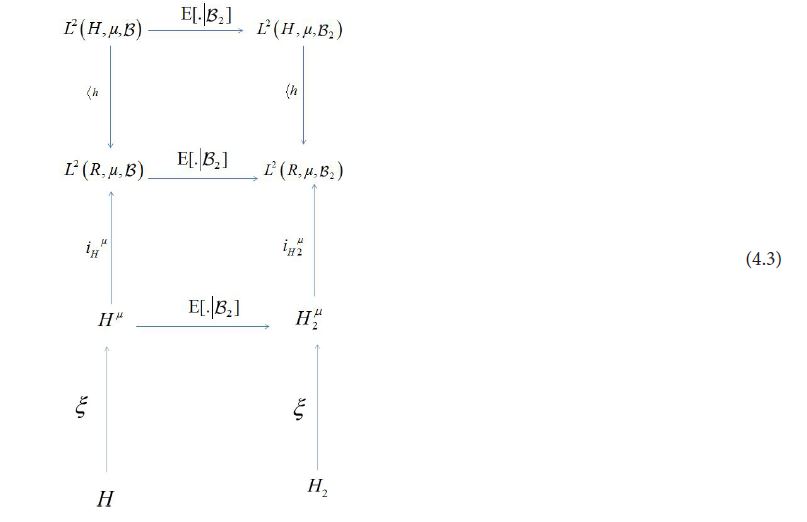
Although there is a natural projection map P_H2:H→H₂ for the bottom of this diagram, in general it cannot be inserted here and maintain the commutativity of the diagram. This comes from the fact that there may exist an hH such that ξ_h = 0. However, this does not imply that .

We are now prepared to obtain the main assertion. The covariance operator of the random variable X is defined by

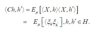
Moreover, by the theorem of normal correlation and the commutativity of the diagram (4.1), the conditional covariance operator is defined by

In terms of the Gaussian Hilbert spaces using the commutativity of the diagram (4.2) and the identification of the conditional expectation with orthogonal projection, we conclude that

and

Since the orthogonal projection p_H^μ2 is a metric projection of H^μonto,H^μ₂ we can express the dual optimization problem to the metric projection as follows: for any hH, using the decomposition h=h₁ +h₂ with h₁H₁,h₂H₂,we decompose Then, noting that we obtain

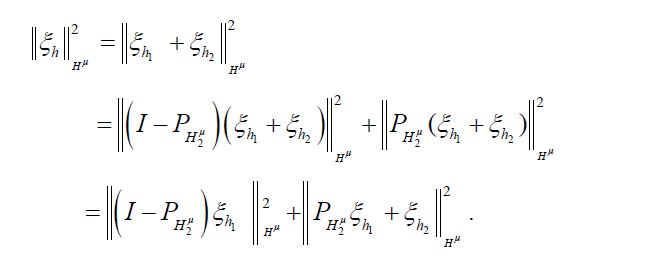
Since in the second term on the right-hand side there is a sequence h₂ⁿ,n=1,..... such that the corresponding sequence converges to and therefore H^μ, we conclude that

From the identifications (4.4) and (4.5), we conclude that

Therefore, Anderson and Trapp implies the assertion

The assertion in the non-centered case follows by simple translation.

Proof of Theorem 3.1 Since the range of is finite dimensional, and therefore closed, so that it follows from Corach, Maestripieri and Stojanoff that An is compatible with H₂ for all n. Now we utilize the approximation results of Butler and Morley for the shorted operator. By their Lemma 1, for cH and for fixed n, it follows that there exists a sequence and a real number M such that

Since this can be written as

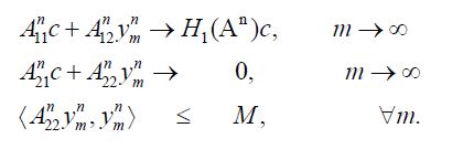
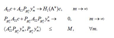
Since these equations only depend on we can further assume that where is the orthogonal projection onto That is, we can assume that and therefore

It follows from for the unique square root. Consequently, it follows that for all n and sincefor all n it follows that for all n. Consequently, the sequence is bounded. Therefore there exists a weakly convergent subsequence. Let n′ denote the index of any weakly convergent subsequence, so that

for some d^' depending on the subsequence. Now the strong convergence of the lefthand side to the righthand side in (4.6) is maintained for the subsequence n^' and, since for the subsequence the first term on the righthand side converges weakly to d′, it follows that we can define a monotonically increasing function m(^n') and use it to define a new sequence such that

Since is strongly convergent to P_H2 it follows that is strongly convergent to P_H2 , so that converges to and converges to -A₂₁c Moreover, by Reid’s inequality, Corollary 2, we have

for all n^',so that the sequence is bounded. Since weak convergence of a bounded sequence on a separable Hilbert space is equivalent to the convergence with respect to each element of any orthonormal basis, it follows that is weakly convergent to -A₂₁c. From (4.8), we obtain

From Kakutani’s generalization of the Banach-Saks Theorem it follows that we can select a subsequence `n of n′ such that the Cesaro means of converge strongly in (4.10). That is, if we consider the Cesaro means

we have

Since A₂₂≥0 it follows that the function is convex, so that for all `n, so that

It therefore follows from Theorem 1 of Butler and Morley that

Consequently, by (4.7), we obtain that

Since this limit is independent of the chosen weakly converging subsequence, it follows that the full sequence weakly converges to the same limit, that is we have

and since c was arbitrary we conclude that

Proof of Theorem 3.3 Let us first establish the assertion when C is compatible with H₂. Consider the operator defined by

Since C is compatible with H₂, there exists an oblique projection QP(C,H₂), and Proposition 4.2 of Corach, Maestripieri and Stojanoff asserts that for E := 1−Q, we have

Since Q^*C =CQ it follows that E^*C =CE, and since Q is a projection, it follows that QE =EQ= 0 and that E is a projection. Moreover, since R(Q) = H₂ it follows that ker(E) = H₂, so that we obtain P₂Q=Q and EP₁ =E and therefore Q^*P₂ =Q^* and P₁E^* =E^* . Consequently, we obtain

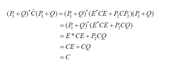
Since Q is a projection onto H₂, it follows that P₁+Q is lower triangular in its partitioned representation and therefore the fundamental pivot produces an explicit, and most importantly continuous, inverse. Indeed, if we use the partition representation

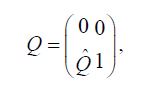
we see that

from which we conclude that

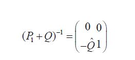
Without partitioning, using P₁Q= 0 and QP₂ =P₂, we obtain

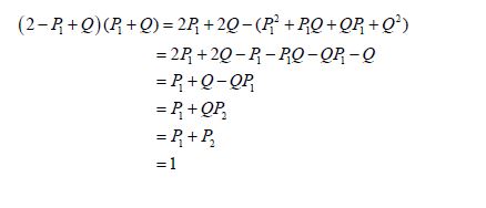
and so confirm that

Following the proof of Lemma 4.3 of Hairer, Stuart, Voss, and Wiber, let N (m,C) denote the Gaussian measure with mean m and covariance operator C and consider the transformation

where we use the notation A^−* for (A⁻¹ )^* = (A^*)⁻¹ . From (4.14) we obtain

so that the transformation law for Gaussian measures, see Lemma 1.2.7 of Maniglia and Rhandi, implies that

Since

we obtain

and therefore

Since the partition representation of

the components of the corresponding Gaussian random variable are uncorrelated and therefore independent. That is, we have

This independence facilitates the computation of the conditional measure as follows. Let X = (X₁,X₂) denote the random variable associated with the Gaussian measure N (m,C) and consider the transformed random variable Y = (P₁+Q)^−*X with the product law.

then,

can be used to compute the conditional expectation as

obtaining

so that we conclude that

A similar calculation obtains the covariance

thus establishing the assertion in the compatible case.

For the general case, we do not assume that C is compatible with H₂. Consider an ordered orthonormal basis for H₂, let H₂ⁿ denote the span of the first n basis elements, let denote the orthogonal projection onto and consider the sequence of Gaussian measures with the mean Pⁿm and covariance operators

As asserted in Theorem 3.1, Cn is compatible with H2 for all n, and the sequence H₁(Cⁿ) converges weakly to H₁(C). Let c(X₁|H₂ⁿ) and C(X₁|X₂) denote the conditional covariance operators associated with the measure μ. Then we will show that c(X₁|H₂ⁿ)=H₁(cⁿ)so that the assertion regarding the conditional covariance operators is established if we demonstrate that the sequence of conditional covariance operators c(X₁|H₂ⁿ) converges weakly to C(X₁|X₂).

To both ends, consider the Lebesgue-Bochner space L²(H,μ,) space of (equivalence classes) of H-valued Borel measurable functions on H whose squared norm

is integrable. Since Fernique’s Theorem, implies that the random variable X is square Bochner integrable, it follows that the Gaussian random variables PⁿX are also square Bochner integrable with respect to μ. Let us denote and and let denote the image under the projection. μ_n is a Gaussian measure on H with mean Pⁿm and covariance Cⁿ.

Now consider a function f: H →H which is Bochner square integrable with respect to μ and satisfies f oPⁿ =f. Then, using the change of variables formula for Bochner integrals, see Theorem 2 of Bashirov, et al. along with the fact that and using the fact that for an arbitrary measurable function g we have g =g^oPⁿ, it follows that for we have

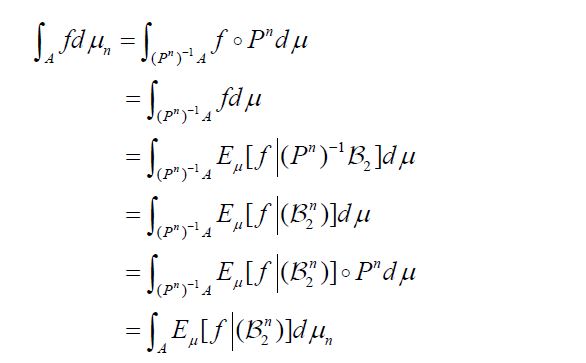
we obtain

and conclude that the sequence is a martingale corresponding to the increasing family of σ-algebras . Moreover, it is easy to see that (4.19) holds for real valued functions f: H →R which are square integrable with respect to μ and satisfy f f^oPⁿ =f. With the choice f:= X₁, we clearly have X₁^oPⁿ = X₁, so that if we denote X₂ⁿ:=PⁿX₂ we conclude that the sequence

is a martingale. Since conditional expectation is a contraction, it follows that the L² norm of all the conditional expectations are uniformly bounded by the L² norm of X. Then by the Martingale Convergence Theorem, Corollary V.2.2 of Diestel and Uhl, For the conditional covariance operators, observe that (4.20) implies that

for all n, so that for h₁,h₂ H, we have

and since the integrand it follows from (4.19) that

so that using the theorem of normal correlation, we obtain

Since the theorem of normal correlation also shows that

the difference in the covariances can be decomposed as

where the last term can be decomposed as

Then since conditional expectation is a contraction on L₂(H,μ,) it follows thatfor all n. Moreover, sinceconvergesit follows thatfor all hH. Therefore, the Cauchy-Schwartz inequality applied four times in the above decomposition implies that

so that we obtain

Since Cⁿ is compatible with H₂ for all n, and the compatible case demonstrated in (4.18) that

for all n, and Theorem 3.1 asserts that

we conclude that establishing the assertion regarding the covariance operators.

For the means, observe that since μ is a probability measure, it follows that X and therefore X₁lie in the Lebesgue-Bochner space L¹(H,μ, ), and since by Diestel and Uhl the conditional expectation operators are also contractions on L1(H,μ,) it also follows that converges to E_μ[X₁|X₂] in L¹(H,μ,). Therefore, Diestel and Uhl [13, Thm. V.2.8] implies that converges to E_μ[X₁|X₂] a.e.-μ. Let the conditional means E_μ[X₁|X₂]be denoted by E_μ[X₁|X₂]=m_t,tH₂Then, since

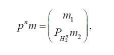
is the mean of the measure μn, the assertion in the compatible case demonstrated that the conditional means =m_tⁿ,tH₂are

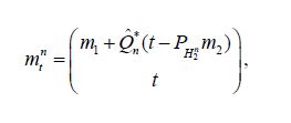
Since the conditional meansconverge to the conditional means E_μ[X₁|X₂]i.e.-μ amounts to m_tⁿ→m_t for μ-almost every t, the first assertion regarding the means is also proved. Now suppose that Qn eventually becomes the special elementdefined near (3.2). Then, by definitionand thereforeso that the final assertion follows from the previous.

Proof of Corollary 3.4 By Mourier’s Theorem, there exists a Gaussian measure μ on H with mean 0 and covariance operator C :=A. Looking at the end of the proof of Theorem 3.3, since conditional expectation is a contraction on L₂(H,μ,) it follows thatfor all n. Therefore, for hH, it follows from the Cauchy-Schwartz inequality thatfor all n, uniformly for hH with ||h||_H≤1Therefo the Cauchy-Schwartz inequality applied four times in the decomposition at the end of the proof of Theorem 3.3 implies that

Uniformly for Therefore, it follows that the sequence of covariance operators converges

in the uniform operator topology.

According to Maniglia and Rhandi or Da Prato and Zabczyk, for a Gaussian measure μ with mean 0 and covariance operator C, we have

From (4.22), by shifting to the center, we obtain that

And

and therefore the difference

Therefore, the Cauchy-Schwartz inequality, the L² convergence of E_μ[X₁|X₂ⁿ] to E_μ[X₁|X₂], and the uniform L₂ boundedness of E_μ[X₁|X₂ⁿ] E_μ[X₁|X₂] and X₁, implies that

Since in the uniform operator topology, it follows from Kubrusly that in the trace norm topology. Since (4.23) asserts that and Theorem 3.3 asserts that the identification A:=C completes the proof [40-46].

The authors gratefully acknowledge this work supported by the Air Force Office of Scientific Research under Award Number FA9550-12-1-0389 (Scientific Computation of Optimal Statistical Estimators).



x1. Krein M (1947) The theory of self-adjoint extensions of semi-bounded hermitian transformations and its applications. I Matematicheskii Sbornik 62: 431-95.

x2. Anderson WN, Trapp GE (1975) Shorted operators. II. SIAM J Appl Math 28: 60-71.

x3. Hairer M, Stuart AM, Voss J, Wiberg P (2005) Analysis of SPDEs arising in path sampling. Part I: The Gaussian case. Commun Math Sci 3: 587-603.

x4. Stuart AM (2010) I nverse problems: a Bayesian perspective. Acta Numer 19: 451-559.

x5. Dalecky YL, Fomin SV (1991) Measures and Differential Equations in Infinite-dimensional Space. Springer Science & Business Media 76.

x6. Mandelbaum A (1984) linear estimators and measurable linear transformations on a Hilbert space. J Prob Theor Relate Area 65: 385-97.

x7. LaGatta T (2013) Continuous disintegrations of Gaussian processes. Theory Probab Appl 57: 151-62.

x8. Tarieladze V, Vakhania N (2007) Disintegration of Gaussian measures and average-case optimal algorithms. J Complex 23: 851-66.

x9. Lee D, Wasilkowski GW (1986) Approximation of linear functionals on a Banach space with a Gaussian measure. J Complex 2: 12-43.

x10. Traub JF, Wasilkowski GW, Wozniakowski H (1998) Information-Based Complexity. Academic Press, New York.

x11. Diaconis P (1988) Bayesian numerical analysis. In Statistical Decision Theory and Related Topics 1: 163-75.

x12. Poincare H (1896) Calculation of probabilities. Georges Carr’es, Paris.

x13. Sul’din AV (1959) Wiener measure and its applications to approximation methods. I Izv Vyss Ucebn Introduced. Mathematics 1959: 145-58.

x14. Larkin FM (1972) Gaussian measure in Hilbert space and applications in numerical analysis. Rocky Mountain J Math 2: 379-422.

x15. Sard A (1963) Linear approximation. American Mathematical Society, Providence.

x16. Kimeldorf GS, Wahba G (1970) A correspondence between Bayesian estimation on stochastic processes and smoothing by splines. Ann Math Statist 41: 495–502.

x17. Shaw JEH (1988) A quasirandom approach to integration in Bayesian statistics. Ann. Statist., 16: 895-914.

x18. O’Hagan A (1992) Some Bayesian numerical analysis. In Bayesian Statistics, Oxford Univ Press, New York 345-63.

x19. Briol FX, Cockayne J, Teymur O, Yoo WW, Schober M, et al. (2016) Contributed discussion on article by Chkrebtii, Campbell, Calderhead, and Girolami. Bayesian Anal 11: 1285-93.

x20. Owhadi H, Scovel C (2017) Universal scalable robust solvers from computational information games and fast eigenspace adapted multiresolution analysis. arXiv: 1703.10761.

x21. Skilling J (1991) Maximum Entropy and Bayesian Methods: Seattle, chapter Bayesian Solution of Ordinary Differential Equations. Springer Netherlands, Dordrecht.

x22. Schober M, Duvenaud DK, Hennig P (2014) Probabilistic ODE solvers with Runge-Kutta means. Advances in Neural Information Processing Systems 27: 739-47.

x23. Owhadi H (2015) Bayesian numerical homogenization. Multiscale Model Simul 13: 812-28.

x24. Hennig P, Osborne MA Girolami M (2015) Probabilistic numerics and uncertainty in computations. Proc R Soc 471: 20150142.

x25. Hennig P (2015) Probabilistic interpretation of linear solvers. SIAM J Optim 25: 234-60.

x26. Briol FX, Oates CJ, Girolami M, Osborne MA, Sejdinovic D (2015) Probabilistic integration: A role for statisticians in numerical analysis? arXiv: 1512.00933.

x27. Raissi M, Perdikaris P, Karniadakis GE (2017) Inferring solutions of differential equations using noisy multi-fidelity data. J Comp Phy 335: 736-46.

x28. Owhadi H (2017) Multigrid with rough coefficients and multiresolution operator decomposition from hierarchical information games. SIAM Rev 59: 99-149.

x29. Cockayne J, Oates CJ, Sullivan T, Girolami MA (2016) Probabilistic meshless methods for partial differential equations and Bayesian inverse problems. arXiv: 1605.07811.

x30. Perdikaris P, Venturi D, Karniadakis GE (2016) Multifidelity information fusion algorithms for high-dimensional systems and massive data sets. SIAM J Sci Comput 38: 521-38.

x31. Sch¨afer F, Sullivan TJ Owhadi H (2017) Compression, inversion, and approximate PCA of dense kernel matrices at near-linear computational complexity. arxiv.org/abs/1706.02205.

x32. Owhadi H, Scovel C (2019) Operator Adapted Wavelets, Fast Solvers, and Numerical Homogenization: from a game theoretic approach to numerical approximation and algorithm design.

x33. Da Prato G, Zabczyk J (2014) Stochastic Equations in Infinite Dimensions. Cambridge University press 152.

x34. Vakhania N, Tarieladze V, Chobanyan S (1987) Probability distributions on Banach spaces, Springer Science & Business Media 14.

x35. Dudley RM (1989) Real Analysis and Probability, Cambridge Studies in Advanced Mathematics. Cambridge University Press, Cambridge 74.

x36. Bogachev VI (1998) Gaussian Measures. American Mathematical Soc 62: 1-90.

x37. Diestel J, Uhl JJ (1977) Vector measures. Number 15 in Mathematical Surveys and Monographs. Am Math Soc 15: 1.

x38. Corach G, Maestripieri A, Stojanoff D (2001) Oblique projections and Schur complements. Acta Sci Math 67: 337–56.

x39. Janson S (1997) Gaussian Hilbert Spaces. Cambridge University Press 129.

x40. Corach G, Maestripieri A, Stojanoff D (2006) Projections in operator ranges. Proceedings of the American Mathematical Society 134: 765–78.

x41. Butler CA, Morley TD (1988) A note on the shorted operator. SIAM J Matrix Anal Appl 9: 147-55.

x42. Reid WT (1951) Symmetrizable completely continuous linear transformations in Hilbert space. Duke Math J 18: 41-56.

x43. Maniglia S, Rhandi A (2004) Gaussian measures on Hilbert spaces. Quaderni of the Department of Mathematics of the University of Salento 2004: 1-24.

x44. A Bashirov (2003) Partially Observable Linear Systems under Dependent Noises. Birkh¨auser Verlag.

x45. Kubrusly CS (1986) On convergence of nuclear and correlation operators in Hilbert space. Mat Apl Comput 5: 265-82.

x46. Kakutani S (1938) Weak convergence in uniformly convex spaces. Tˆohoku Math J 45: 188-93.

x

3. Hairer M, Stuart AM, Voss J, Wiberg P (2005) Analysis of SPDEs arising in path sampling. Part I: The Gaussian case. Commun Math Sci 3: 587-603.

4. Stuart AM (2010) I nverse problems: a Bayesian perspective. Acta Numer 19: 451-559.

5. Dalecky YL, Fomin SV (1991) Measures and Differential Equations in Infinite-dimensional Space. Springer Science & Business Media 76.

x

6. Mandelbaum A (1984) linear estimators and measurable linear transformations on a Hilbert space. J Prob Theor Relate Area 65: 385-97.

7. LaGatta T (2013) Continuous disintegrations of Gaussian processes. Theory Probab Appl 57: 151-62.

8. Tarieladze V, Vakhania N (2007) Disintegration of Gaussian measures and average-case optimal algorithms. J Complex 23: 851-66.

9. Lee D, Wasilkowski GW (1986) Approximation of linear functionals on a Banach space with a Gaussian measure. J Complex 2: 12-43.

10. Traub JF, Wasilkowski GW, Wozniakowski H (1998) Information-Based Complexity. Academic Press, New York.

x

10. Traub JF, Wasilkowski GW, Wozniakowski H (1998) Information-Based Complexity. Academic Press, New York.

11. Diaconis P (1988) Bayesian numerical analysis. In Statistical Decision Theory and Related Topics 1: 163-75.

12. Poincare H (1896) Calculation of probabilities. Georges Carr’es, Paris.

13. Sul’din AV (1959) Wiener measure and its applications to approximation methods. I Izv Vyss Ucebn Introduced. Mathematics 1959: 145-58.

14. Larkin FM (1972) Gaussian measure in Hilbert space and applications in numerical analysis. Rocky Mountain J Math 2: 379-422.

15. Sard A (1963) Linear approximation. American Mathematical Society, Providence.

16. Kimeldorf GS, Wahba G (1970) A correspondence between Bayesian estimation on stochastic processes and smoothing by splines. Ann Math Statist 41: 495–502.

17. Shaw JEH (1988) A quasirandom approach to integration in Bayesian statistics. Ann. Statist., 16: 895-914.

18. O’Hagan A (1992) Some Bayesian numerical analysis. In Bayesian Statistics, Oxford Univ Press, New York 345-63.

x

19. Briol FX, Cockayne J, Teymur O, Yoo WW, Schober M, et al. (2016) Contributed discussion on article by Chkrebtii, Campbell, Calderhead, and Girolami. Bayesian Anal 11: 1285-93.

20. Owhadi H, Scovel C (2017) Universal scalable robust solvers from computational information games and fast eigenspace adapted multiresolution analysis. arXiv: 1703.10761.

21. Skilling J (1991) Maximum Entropy and Bayesian Methods: Seattle, chapter Bayesian Solution of Ordinary Differential Equations. Springer Netherlands, Dordrecht.

22. Schober M, Duvenaud DK, Hennig P (2014) Probabilistic ODE solvers with Runge-Kutta means. Advances in Neural Information Processing Systems 27: 739-47.

23. Owhadi H (2015) Bayesian numerical homogenization. Multiscale Model Simul 13: 812-28.

24. Hennig P, Osborne MA Girolami M (2015) Probabilistic numerics and uncertainty in computations. Proc R Soc 471: 20150142.

25. Hennig P (2015) Probabilistic interpretation of linear solvers. SIAM J Optim 25: 234-60.

26. Briol FX, Oates CJ, Girolami M, Osborne MA, Sejdinovic D (2015) Probabilistic integration: A role for statisticians in numerical analysis? arXiv: 1512.00933.

27. Raissi M, Perdikaris P, Karniadakis GE (2017) Inferring solutions of differential equations using noisy multi-fidelity data. J Comp Phy 335: 736-46.

28. Owhadi H (2017) Multigrid with rough coefficients and multiresolution operator decomposition from hierarchical information games. SIAM Rev 59: 99-149.

29. Cockayne J, Oates CJ, Sullivan T, Girolami MA (2016) Probabilistic meshless methods for partial differential equations and Bayesian inverse problems. arXiv: 1605.07811.

30. Perdikaris P, Venturi D, Karniadakis GE (2016) Multifidelity information fusion algorithms for high-dimensional systems and massive data sets. SIAM J Sci Comput 38: 521-38.

31. Sch¨afer F, Sullivan TJ Owhadi H (2017) Compression, inversion, and approximate PCA of dense kernel matrices at near-linear computational complexity. arxiv.org/abs/1706.02205.