Perceptive Response on Solid Waste Management and Willingness to Pay at Bhairahawa and Butwal, Nepal
Majority of cities of Nepal including Bhairahawa and Butwal are facing serious problems in managing municipal wastes. It is seriously constrained by budgetary problems and other managerial aspects. In this regard, this study was designed to record the perception of people in these two cities regarding various aspects of solid waste management. To elicit willingness to pay, single bounded dichotomous choice contingent valuation method was employed. Study was based on 100 respondents, 50 from each site. Out of total respondents, 72.8 percent were willing to pay for improved solid waste management. People from Butwal are more willing to pay in this regard. Moreover, they are more engaged in proper waste management as well as compared to Bhairahawa. Result revealed that location, salary, family size, ethnicity and level of education are the factors affecting willingness to pay for improved solid waste management. Currently, respondents from Butwal are paying $ 0.24/week for waste management whereas respondents from Bhairahawa are not paying a penny. So, there is the opportunity of increasing garbage fee the present garbage fee is far below the mean willingness to pay of households. The mean willingness to pay may be a guide to municipal authorities to determine appropriate garbage fee. The findings may serve as a guide to act for better solid waste management in the study area.
Keywords: Waste; Willingness to pay; Management
Solid waste refers to any garbage, trash or refuses which are in solid form [1]. Municipal solid wastes refer to the heterogeneous form of solid wastes collected in urban areas. Solid wastes management problems are growing in developing countries because of growing population. The average municipal budget spent on solid waste management is only about 10% and only 62.3% of the total municipal waste generated is collected by the municipalities in Nepal [2]. The Solid Waste Management (SWM) Act of 2011 was enacted by the Government of Nepal gave full responsibility to municipalities for the SWM service but, progress in this regard is very minimal [ 3]. Two growing cities, Siddhartha agar municipality (popularly known as Bhairahawa) and Butwal sub metropolitan city were purposively selected for the purpose of this study to assess the perception of residents regarding various aspects of solid waste management and willingness to pay for better management of it. Butwal is the capital of newly formed province no .5 of Nepal (name is yet to be finalized) and Bhairahawa is the one of the main gateway to Nepal. Waste management is a serious problem in these areas and no any studies and intervention is done in the selected area. These two cities are 22 km apart with different kind of societal set up.
For this study, contingent valuation method was used to elicit the willingness to pay (WTP) by the households in Butwal and Bhairahawa for effective solid waste management. The choice of this method was done as this method directly reports the willingness to pay of people to obtain a specified good and/or service, or willingness to accept to give up a good and/or service, rather than inferring them from observed behaviors in regular market places for betterment of environmental components. Checklists were prepared according to [4].
Vicinity at around Dande River, Bhairahawa and Tinau River, Butwal were purposively selected for the purpose as solid wastes are dumped in the bank of these rivers. People living near to the dumping sites were selected as respondents.
Both primary and secondary data were collected during the study. Primary data collection methods were basically questionnaire and focused group discussion. 100 respondents were selected, 50 from each location based on simple random sampling. Questionnaires were discussed with experts and were pre-tested before finalizing it. The survey was conducted using the face-to-face interview method, which is considered to produce the highest quality and the most reliable WTP data [5]. A semi-structured questionnaire was used to collect data from the households including questions related to the demography, socioeconomic characteristics, and current scenario of solid waste and its management, their perceptions, services provided by the municipality regarding solid waste management, level of awareness and questions related to willingness to pay. In order to elicit the maximum WTP amount for improved waste collection service, an open-ended contingent valuation method was used in this study. In the present context, it is the most informative and supposedly superior elicitation technique [6]. The current solid waste collection charge was taken as a base value and was subsequently increased using this technique until the respondents gave positive response on willingness to pay.
SPSS version 22 was used for data entry and analysis. Chi square test was used for testing of significance. Bar diagram was then constructed using MS-EXCEL. Secondary data regarding the available services was collected from the district offices and internet. Moreover, the river water samples were collected from the selected ten locations as per standard sampling methods. Five were regarded as upstream and five as downstream based on the dumping site location. Observations were recorded for the analysis of parameters like temperature, pH, dissolved oxygen and turbidity. Each analysis was done in triplicate and the mean value was taken.
The mean age of respondents at Butwal was 45 years old with predominantly female (62% ) whereas, in Bhairahawa it was and that in case of Butwal was 51 years and predominantly male (75.3% ). The average size of the household of respondent is 5.34 in case of Butwal whereas 5.69 in case of Bhairahawa. The average monthly household income is found to be NRs. 16,854.20 in case of Bhairahawa whereas 22,460.60 in case of Butwal. 5.7% people from Bhairahwa are engaged in agriculture, 18.9% are engaged in business, 9.4% have government job, 7.5% from remittance, 58.5% have non-governmental job. However, in Butwal, 2%, 62%, 6%, 12% and 18% respondents’ main source of income is agriculture, business, remittance, non-governmental jobs and others respectively. The difference was found significant (X2=41.48, P<0.001) (Figure 1).
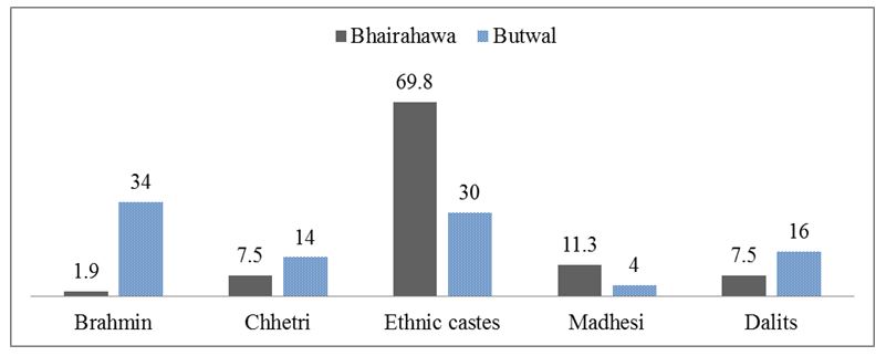
There existed significant difference in the ethnicity of respondents (X2=27.6, P< 0.000) in the study site. In close to periphery of Dande river, Bhairahawa where the study was conducted, there is dense population of Janajatis (ethnic castes) followed by Madhesis. However, in case of Butwal population of Bhramins (upper caste) was more followed by ethnic castes and Dalits (lower castes) (Figure 2).
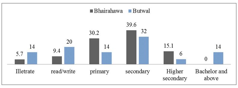
Upon analysis of education of respondents, significant difference (X2=27.4, P< 0.000) was observed in these two locations. Respondents with education of Bachelor or above were not seen in case of Bhairahawa. Majority of respondents in both the cases were with secondary level of education.
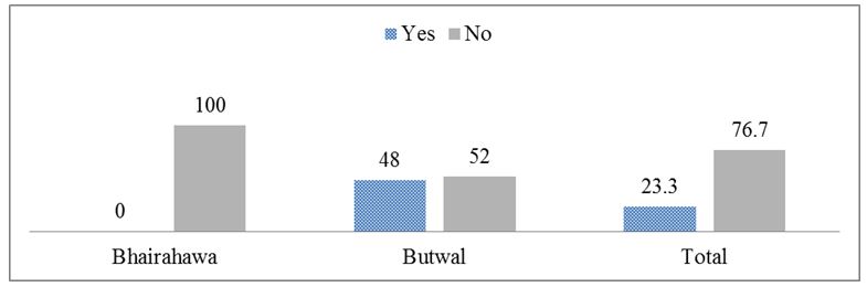
Every respondents from Bhairahawa were not paying a penny where as 48% respondents from Butwal were charged for waste pickup and the response was found to be significantly different (X2=33 P< 0.001). At present the respondent of Butwal are paying Rs. 100 per month (approximately $0.9) (Figure 3).
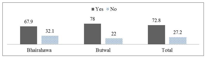
72.8% of total respondents were willing to pay for better solid waste management. Though the percentage of respondents who are willing to pay was higher in case of Butwal (78%) as compared to Bhairahawa (67.9%), no any significant difference in response was noted. The mean willingness to pay amount for Bhairahawa was Rs. 70.57 ($0.65), whereas that of Butwal was Rs. 120 ($1.11) per household. This share of respondents’ WTP is somewhat similar to other similar studies where more than 60% of the respondents provided a positive response [7] (Figure 4). When asked about the reasons of their willingness to pay for better solid waste management, the reasons mentioned by them is summarized as under:
• To maintain and recover their surrounding cleanliness (90%).
• Regular and proper disposal of wastes 80%).
• Willing to share the cost for effective waste management (25%).
• Willing to pay for the waste collection service as they are devoid of such a service (52%).
Moreover, 27.2% of total respondents were not willing to pay for this purpose. When asked about the reasons, they responded as under:
• It is government duty; they need not to pay for it (80%).
• They pay municipal tax so it should be free (80%).
• Household income is less (70%).
• Can manage by them as they are generating too less waste (22%).
When asked if they are willing to pay Rs. 150 per month and above, following response was obtained:
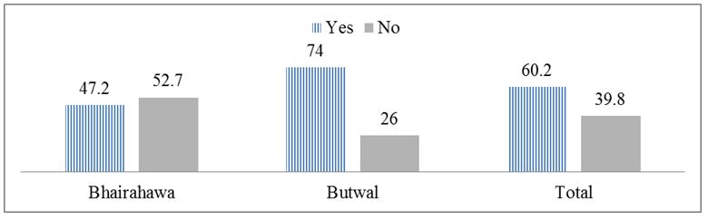
60.2% of respondents are willing to pay Rs. 150/month for solid waste pickup. However, 53.7% respondents from Bhairahawa are not willing to pay this much. 74% respondents from Butwal are willing to pay Rs. 100 per month for better solid waste management as shown in (Figure 5). The response was found to be significantly different (X2=12.73, P< 0.01).
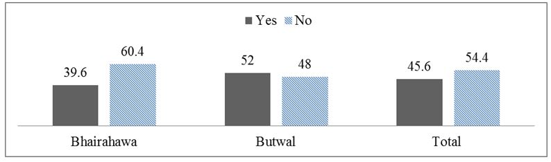
When the bid price was increased to Rs. 200 per month, majority of respondents (54.4%) are not willing to pay further for waste pickup. The percentage of respondents from Bhairahawa who are not willing to pay is more than that of Butwal as shown in (Figure 6). The response in case of Bhairahawa and Butwal was not significantly different.
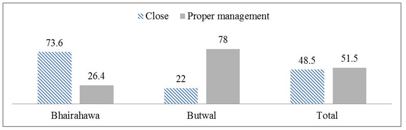
Significant difference was noted (X2=27.4, P< 0.001) in the response on what is to be done on existing dumping site. 73.6% respondents from Bhairahawa said that the dumping site is to be closed soon while 26.4% said proper management is to be done. However, only 22% respondents from Butwal voted for closure of existing dumping site and 78% said that it should be properly managed rather than closing it (Figure 7).
Effect of Improper Solid Waste Management: Improper waste disposal seems to influence significantly in the agricultural production and increase disease incidence. Response of effect on agricultural production was significantly affected by the location of respondents and their education level. People form Bhairahawa felt significantly that the waste has declined agricultural production in comparison to that of Butwal. In comparison to poorly educated people, highly educated people felt that the waste disposal have declined agricultural productivity. The model chi square was significant at P<0.001 (X2=35.072). In contrary to this, people from Butwal feels 65% more that waste disposal have increased the incidence of disease and the response was significant (p<0.05). Income of respondents also seems to increase the response in this regard. The model was fit in this case as well (model X2=14.81, p<0.05) (Table 1).
Factors Influencing Reuse, Recycle and Reduction of Wastes: The results from the logit regression model for reuse, recycling and reduction of wastes are presented in table below. The model chi square was significant for whether the respondents reuse or recycle the waste at least periodically to some extent. When explored for reuse of wastes, 63% of cases were correctly classified.
The Table showed that reuse of waste is significantly affected by education level and family size. It highlighted that people with higher education tend significantly to reuse. Moreover, recycling is affected by address of respondents. People from Butwal are 89.8% more likely to recycle the wastes as compared to Butwal and the case is 81% correctly classified. The model of fit is good in both the cases (for reuse at p<0.05 and for recycling of waste at p<0.01).
Factors influencing willingness to pay: 73% of cases are correctly classified for willingness to pay. As respondents from both location are willing to pay no such significant difference was noted. However, model for willingness to pay @Rs. 100/month was found to be significant at p<0.001(chi square=30.731). 75% cases were correctly predicted. People from Butwal are more willing to pay at Rs. 100 per month. Thus, the validity of the logit model to estimate determinants of is consistent with other similar studies.
Factors influencing waste segregation and other alternatives: Waste segregation is more followed in case of Bhairahawa as compare to Butwal. Net of other factors, the finding was significant (model X2=11.74, p<0.05). Alternative dumping at Butwal is significantly higher in comparison to Bhairahawa (P<0.001). It is done significantly highly by marginalized groups as compared to elite group (P<0.05). In this case, 73% cases are correctly predicted and model chi square was significant (model X2=27.34, P<0.001). Surprisingly alternative burning of waste was more followed by highly educated respondents (model X2=11.34, P<0.05). Similarly, alternative composting was significantly highly practiced by people with low education (P<0.05) but the model chi square was not significant.
Moreover, water quality at both the sites was also checked. Each site was demarked as upstream and downstream based on the location of dumping site. Five spots were selected at each site. Spots before the dumping site were regarded as upstream and spots after dumping site were regarded as downstream. Based on the study, following observations are presented at Tables 5 and 6.
According to Table 5, any significant difference was noted in pH and temperature. The dissolved oxygen of upstream in Dande River, Bhairahawa was significantly higher as compared to downstream. The leaching of wastes disposed in the bank of river seems to have decreased the dissolved oxygen. Moreover, the turbidity and total dissolved solids at downstream significantly increased in comparison to upstream due to waste disposal and its leaching into the water body.
In case of Butwal the temperature, turbidity and total dissolved solids at downstream were significantly higher and dissolved oxygen was significantly lower in comparison to upstream. No any significant difference was noted in this case as shown in Table 6.
both of the sites is in the accepted range of 6.5-8.5 as proposed by WHOM, IMCR and BIS. The range of 5-14.5 mg O2 L−1 is found to be suitable for the natural waters depending on turbulence, temperature, salinity, and altitude. In our case both site has DO within this range (i.e. 7-8.5). The turbidity of surface water is usually between 1 NTU and 50 NTU. The turbidity range as given by BIS - IS: 10500 – 2012 is 05 NTU (desirable) and 10 NTU (permissible) for drinking water. The increase of turbidity of water results in interference of the penetration of light. This will damage the aquatic life and also deteriorate the quality of surface water. High values of turbidity minimize the filter runs which cause pathogenic organisms to be more hazardous to the human life. The standard for drinking water is 0.5 NTU to 1.0 NTU. Water of both rivers was found to have higher turbidity than prescribed range.
The improper dumping of solid wastes in the banks of both rivers has found to be significantly affecting the water quality. Waste dumping has significantly lowered dissolved oxygen, increased turbidity and total dissolved solid. If proper management of municipal solid waste is not done sooner then, the condition will be more serious and worsen in days to come. So, proper management to this problem should be done. The similar phenomenon was reported from the water of the Karnafuli River in Bangladesh by [8].
Varied response about solid waste and its management and willingness to pay was obtained from the two locations. Respondents from Butwal are more willing to pay for better solid waste management but respondents from Bhairahawa are concerned for closure of existing dumping site. The major factors that are significantly affecting the people’s practices for solid waste management, its allied problem as well as willingness to pay are location, education, income, number of family, ethnicity and gender. pH, Dissolved Oxygen, Turbidity, Total Dissolved Solid and Temperature were considered to assess the quality of river water. Upstream from dumping site was found to be relatively of superior quality as compared to downstream. Effective program is to be undertaken for better management of existing dumping site and reducing the pollution. As there is the opportunity of collecting sufficient funds for the provision of better solid waste management service, municipality may encourage the private sector to initiate such service. However, municipality itself may also initiate the improved solid waste management service. Similarly, the emphasis should also be given on the environmental education on the people.