Alternative Robust Methods of Multivariate Outlier Detection

A multivariate outlying observation is an amalgamation of infrequent marks on as minimum two or more variables. The purpose of this study is recognition of unusual observations in multivariate dataset engaging several techniques, mainly using Mahalanobis method, Cook’s distance method, Leverage point, DFFITS, Standardized residual, Studentized residual, DFBETAS. Numerous traditional unusual observations detection techniques are established on the sample mean and covariance matrix in common. Nonetheless they do not continuously show outperforms, because they theirself are affected by the outlying observations. Occasionally one outlying observation has veiled the other unusual observations. This is the masking effect of the measures and which have to detect. A suitable technique is accepted to detect the unmasking outlying observation and also to compare the several methods. That’s why we have proposed two robust outlier detection methods: (i) 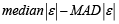And (ii) 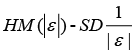. Finally we found that our proposed methods gave the better results than any other methods in versatile aspects.

Keywords: Multivariate Outliers; Outlier Detection Methods; ; ; Simulation Study

Multivariate outlying observation recognition is the vital mission of statistical analysis of multivariate data. Many approaches have been suggested for univariate outlying observation recognition. Identifying outliers in multivariate data pose challenges that univariate data do not discussed in [1]. A multivariate outlying observation need not be an extreme in any of its workings the knowledge of extremeness arises unavoidably form some form of ’ordering’ of the data introduced in [2,3].They are grounded on (robust) estimation of mean and covariance matrix of the data. A key drawback is that these procedures are free from the sample size. The foundation for multivariate outlying observation recognition is the Mahalanobis distance. The usual process for multivariate outlying observation recognition is robust estimation of the parameters in the Mahalanobis distance and the contrast with a critical value of the χ²distribution discussed in [4,5]. Nevertheless, also observations greater than this critical value are not essentially outlying observation; they could quiet fit to the data distribution. The elementary values and difficulties of ‘the ordering of multivariate data’ discussed in [6,7].Attention in outlying observation recognition in multivariate data continued the identical as for the univariate instance. Extreme observations could again deliver indeed interpretable procedures of ecofriendly alarm in their particular correct and if they were not only unusual, but ‘amazingly’ unusual or misleading, they might again recommend that some unexpected impact is current in the data source described in [8,9].So once more we faced the concept of ‘maverick’ or ‘rogue’ unusualness which we would term outlying observation. Thus, as in a univariate sample, an unusual observation may ‘stick out’ so far from the others that it must be affirmed an unusual and a suitable methods of discordance may reveal that it is statistically awkward even when watched as an ‘unusual’. Such an outlying observation is supposed to be conflicting and may lead us to conclude that some anomalies present in the data described in [10,11].The approaches were applied to a set of data to clarify the many outlying observation recognition procedure in multivariate linear regression models. Outliers can misinform the regression results described in [12,13].When an outlying observation is complicated in the study, it drew the regression line towards itself. This could outcome in a explanation that is more exact for the outlying observations, but less accurate for all of the other cases in the data set described in [14,15]. The outlying observation recognition challenge is one of the initial of statistical interests, and since nearly all data sets contain outlying observation of fluctuating ratios, it remains to be one of the most significant. Occasionally outlying observation can totally mislead the statistical analysis, at other times their impact may not be as obvious. Statisticians have consequently established many procedures for the identification and handling of outliers, however most of these approaches were established for univariate data sets. This paper focuses on multivariate outlying observation recognition. Mainly when using some of the general summary statistics such as the location and scale, outlying observation can cause the analyst to influence a decision entirely contrary to the case if outlying observation weren’t present. For instance, a assumption might or might not be avowed significant as a result of a handful of outlying observation. Classical outlying observation recognition is influential when the data hold a single outlier. However, the efficiency of outlier detection methods is decreasing dramatically when the dataset hold more than one outlier. This defeat of accuracy is frequently as a result of what are recognized as the masking difficulties. Furthermore, these approaches do not always flourish in identifying outlying observations. Therefore, a technique which escapes these difficulties is required. How do the outliers occur in the data sets? Outliers can also come in different flavors, depending on the environment: point outliers, contextual outliers, or collective outliers. Most common causes of outliers on data sets are: Data entry error, Appliance errors, planned errors, Data handling errors, Sampling errors and Normal. What are the problems when outlier occurs in the data sets? Outliers have been a major problem in the area of statistics, including modeling, analysis and forecasting. Lots of methods has been portrayed as a means of detecting outliers in multivariate data but not many works has been done on which of this methods is best for detecting outliers in multivariate models. This work addresses that problem by using nine multivariate outlier detection methods and checking which of them is best or more efficient in detecting outliers [16].

Step 1: Run the regression model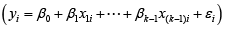
Step 2: Calculate the absolute error of the regression model
Step 3: Calculate median of the absolute error
Step 4: Calculate median absolute deviation (MAD) of absolute error
Step 5: Compute the formula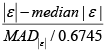
Step 6: Any data value that is greater than is considering being an outlier(s).

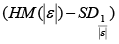
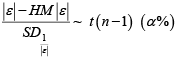
(ii)
Step 1: Run the regression model
Step 2: Calculate the absolute error of the regression model Step 3: Calculate harmonic mean (HM) of the absolute error Step 4: Calculate standard deviation of HM is Step 5: Compute the formula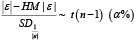
Step 6: Any data value that is greater than
is considering being an outlier.

Here, we have taken two types of outlier detection methods: one is graphical test and another is analytical test. It is very difficult to identify the unusual observations from the graphical methods but we can suspect from the depiction. Most of the researcher used various diagram for outlier detection but we have consider three types of graphs such as scatter diagram, normal QQ plot, and box-plot diagram. Finally, we have tried to detect the actual number of outliers based on analytical methods; the commonly used analytical methods are shown in the Table 1.

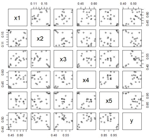
(i) Example 1 In this section, datasets are extracted from [1] which has 20 observations and 6 variables.

Visualization of dataset is very important part of any kinds of analysis. Researchers firstly want to show the data pattern and based on the data pattern they take the decision what they will want to do further. But it is very difficult task sometimes. One of the difficult tasks to detect the outliers in the dataset is very critical. Here, we have considered the graphical methods to suspect the presence and absence of unusual observations in the datasets. This is the preliminary process to progress the work and finally we will apply the analytical methods for outlier detection. The results of the graphical representation are following below-

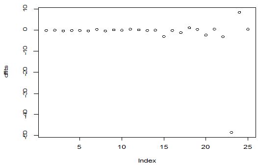
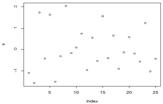
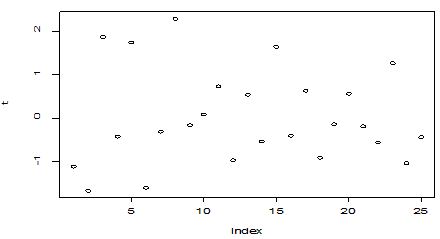
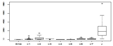
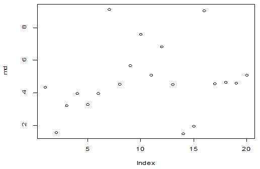
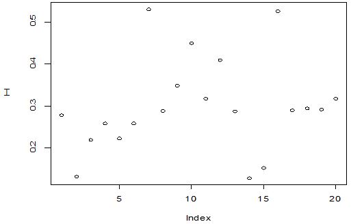
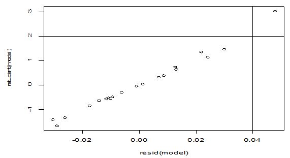
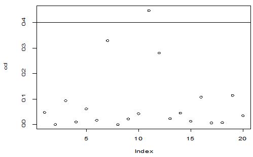
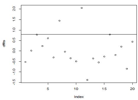
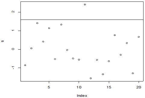
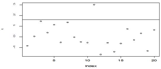
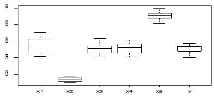
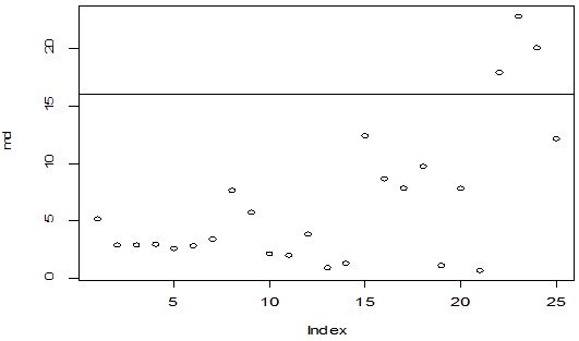
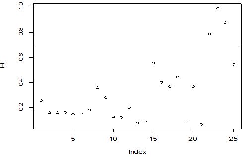
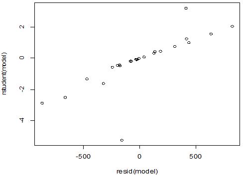
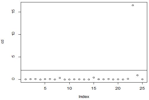
A scatter diagram focuses the data dispersion that means how the data spread from one point to others. However, it is the very simple process to visualize the data pattern.. From Figure 1 we observed that there may have outlier in the dataset. From Figures 2 & 3, it is very clear that there were three outliers in the dataset. From Figure 4, 5, 6, 8 & 9 we observed that there is a single outlier in the dataset. The DEFFITS values in Figure 7 exhibited two outliers. The box-plot diagram is most popular plot to detect the outliers; sometimes it’s called a five number summary. It exhibits the highest value, lowest value, 1st quartile, 2nd quartile and 3rd quartile. Therefore, it is very easy to detect outliers in this way. However, from Figure 10 we showed that there was no outlier in the dataset.

After a primary assessment of outlier revealing is showed with graphical approaches, the ultimate decision on outliers is completed using analytical techniques .The results of the analytical methods are shown in the Table 2.

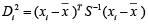
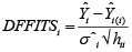
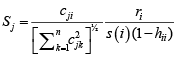
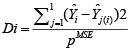
The analytical results in Table 1 deals with the procedure for computing the presence of outliers using various measures such as Mahalanobis Distance (MDi), Cook’s Distance(Di), Leverage point(hii), DFFITS, Standardize residual, Studentized residual and DFBETAS, Proposed method (median|ε|-MAD|ε|) and Proposed method 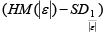. From the dataset, the outlier identification level of Mahalanobis Distance (MDi), Leverage Point (hi), Standardized residual, Cook’s distance and Proposed methods are approximately the same, but DFFITS and DFBETAS outlier detection sensitivity is higher than others methods, since maximum number of outlier points are identified. This result clearly reveals that DFFITS and DFBETAS identify the maximum number of outliers.

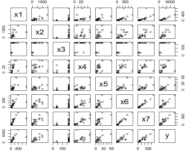
(ii) Example 2 The dataset has taken from [2] which contain 7 independent variables and the response variable y. The result of the dataset is shown in the following below-

In Figure 11 we showed that several pairwise scatter plots indicating the observations with outlying additive outlier value. Figures 12 & 13 depicted three outliers based on Mahalanobis distance values and leverage values. In Figure 14, 15, 16 & 17 displayed single outlier. Alternatively Figures 18, 19 & 20 revealed more than one outlier.

From Table 3 we observed that DFFITS and DFBETAS detected highest number of outliers than all others methods.

Here, we have compared the ability of outlier detection in different methods based on simulation process. We have generated data from a multivariate normal distribution. Firstly, we generate the dataset which is absolutely free from outliers. The results of the study are shown in the Table 4. Secondly we generate the data set which contains outliers. The certain percentage of outlier was casted in the data set at random. In our study, we have taken 5% outliers in data sets of different sizes such as n = 100, 500 and 1000. The results of the simulation study are shown in the following Table 5.

We have taken two categories: one is free from outliers, as presented in Table 4 and for comparison; another is based on 5% contaminations, as presented in Table 5. However, as we have noticed in Table 4 and in our simulations, the methods always yield a massive observations that are (wrongly) specified as outliers except from our proposed two methods but the actual situation is the simulation study was free from contamination. In Table 5 we have displayed the simulation study results of nine methods most of the methods were unable to identify as outliers except only detected our proposed two methods. It is clear that our proposed two methods outperforms considerably with respect to the detection of the accurate outliers. The performance becomes even more obvious as the sample size increases.

To sum up the whole discussion, we have compared the several outlier detection methods such as Mahalanobis Distance (MDi), Cook’s Distance(Di), Leverage point(hii), DFFITS, Standardize residual, Studentized residual, DFBETAS, Proposed method and Proposed method . In this work, the outlier detection way of Mahalanobis Distance (MDi), Leverage Point (hi) and Proposed methods (median|ε|-MAD|ε are approximately the same, this result clearly reveals that DFFITS identify the maximum number of outliers. In this paper we have used several methods for outlier detection. It is very difficult task to recommend one method to detect outlier, because most of the methods have masking and swamping problems in different contexts. Here we can recommend that our proposed two methods may give you a better yield than any other methods.